Overview
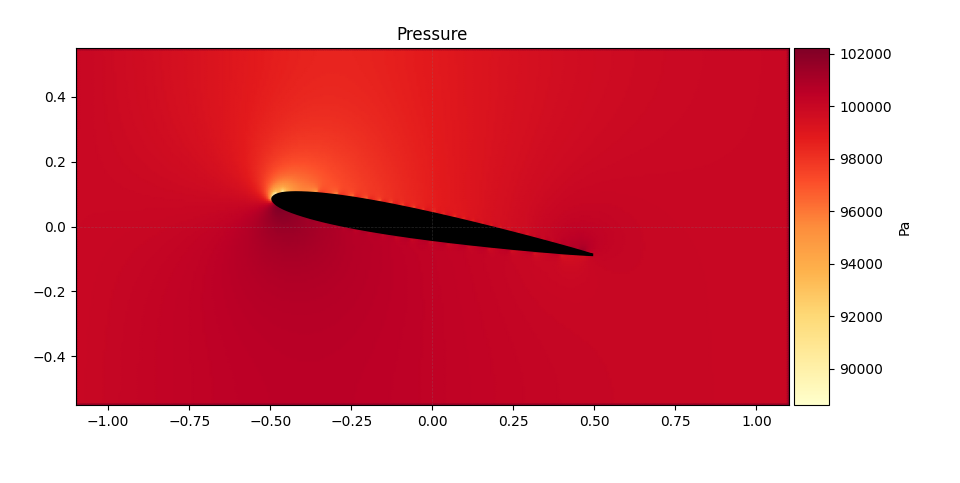
How does air flow around a cylinder, an airfoil, or even a car? We wrote a Python solver that computes the steady, inviscid flow around any two-dimensional body, from simple shapes to outlines traced from a picture, by solving Laplace’s equation for the stream function on a grid. From it come the velocity and pressure fields and the lift, and an interactive window lets you change the shape, the angle of attack and the grid to see how each one changes the flow.
Model and assumptions
The flow is steady, two-dimensional, incompressible and inviscid. Incompressibility lets the velocity be written with a stream function , and for irrotational flow satisfies Laplace’s equation:
The velocity components follow from and , and the pressure from Bernoulli’s equation:
The outer boundaries carry a uniform stream. The body is impermeable, so its wall is a streamline with a constant value of . We used m/s in air at 20 °C, well below Mach 0.3, so the incompressible assumption holds.
Numerical method
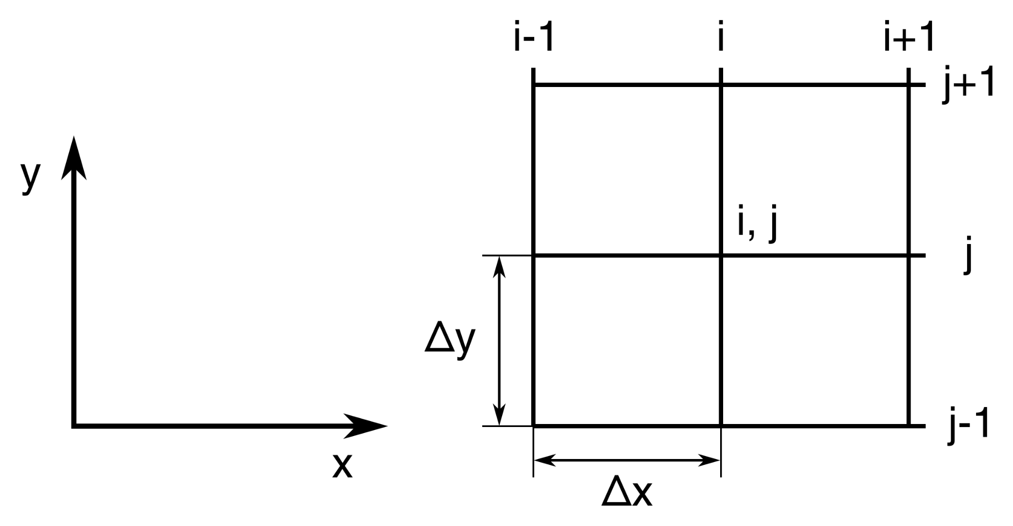
The domain is a Cartesian grid and the body is a mask of grid points. With a centred five-point discretisation and equal spacing in and , each interior value is the mean of its four neighbours:
A Jacobi iteration repeats this update until the largest change falls below a tolerance. The first version ran the loops in plain Python; a later version compiled the iteration and the velocity calculation with Numba and ran the grid rows in parallel, because computation time limited how fine the grid could be. Velocities come from centred differences of . For lift and drag, the pressure field is interpolated onto the body outline and integrated.
The program runs in a Matplotlib window with sliders for the circulation constant, the angle of attack and the grid spacing. It handles a cylinder, a rotating cylinder, a Joukowski airfoil, NACA sections read from coordinate files, and any outline traced from an image.

What the results show
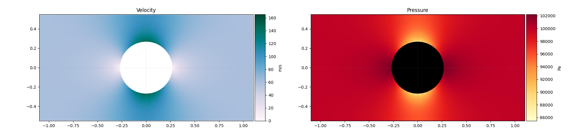
For a cylinder, the solver reproduces the expected picture: symmetric fields and no lift without circulation, and lift in the expected direction once a circulation is added, as for a rotating cylinder.
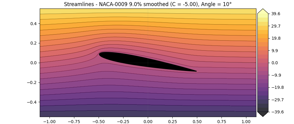
For airfoils, the value of on the body sets the circulation, and nothing in the solver fixes it. In the real flow the Kutta condition picks the one circulation that makes the flow leave the trailing edge smoothly. We knew this, but the code did not impose it: we chose the constant by eye until the streamlines looked right.
| Case | Lift coefficient computed |
|---|---|
| NACA 0009, 5° | 0.203 |
| NACA 0009, 10° | 0.418 |
| NACA 0015, 5° | 0.285 |
| NACA 4415, 5° | 0.719 |
For a thin symmetric section at 5°, thin-airfoil theory gives . The computed values are well below that, which is what a hand-set circulation produces.