Sectorization of the Barcelona FIR

Overview

How should the airspace over Barcelona be divided so that no air traffic controller is overloaded at the busiest time of the morning? We cut the Barcelona flight information region into five sectors drawn by Voronoi diagrams and let a genetic algorithm move their borders to balance the controllers’ workload. After tuning the algorithm with Monte Carlo runs, we compared two ways of trading sector size against the number of aircraft per sector, and found that the multi-objective NSGA-II gave a much fuller picture of the trade-off than a simple weighted sum.

Workload was modelled through the four usual groups of controller tasks: background, transition, recurring and conflict tasks.

Problem setup

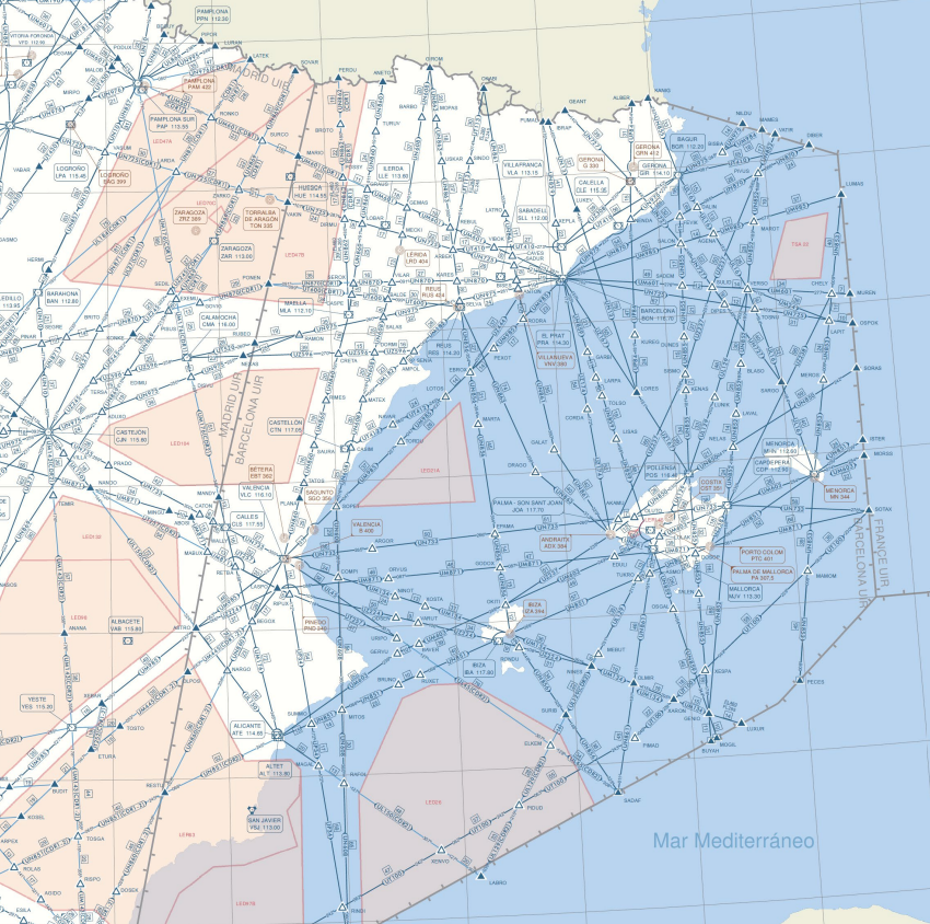
The traffic scenario is the morning peak between 07:55 and 08:10, with 87 flights, from real traffic data supplied by the course. With a limit of about 18 to 19 aircraft per controller, this gives five sectors as the starting configuration.

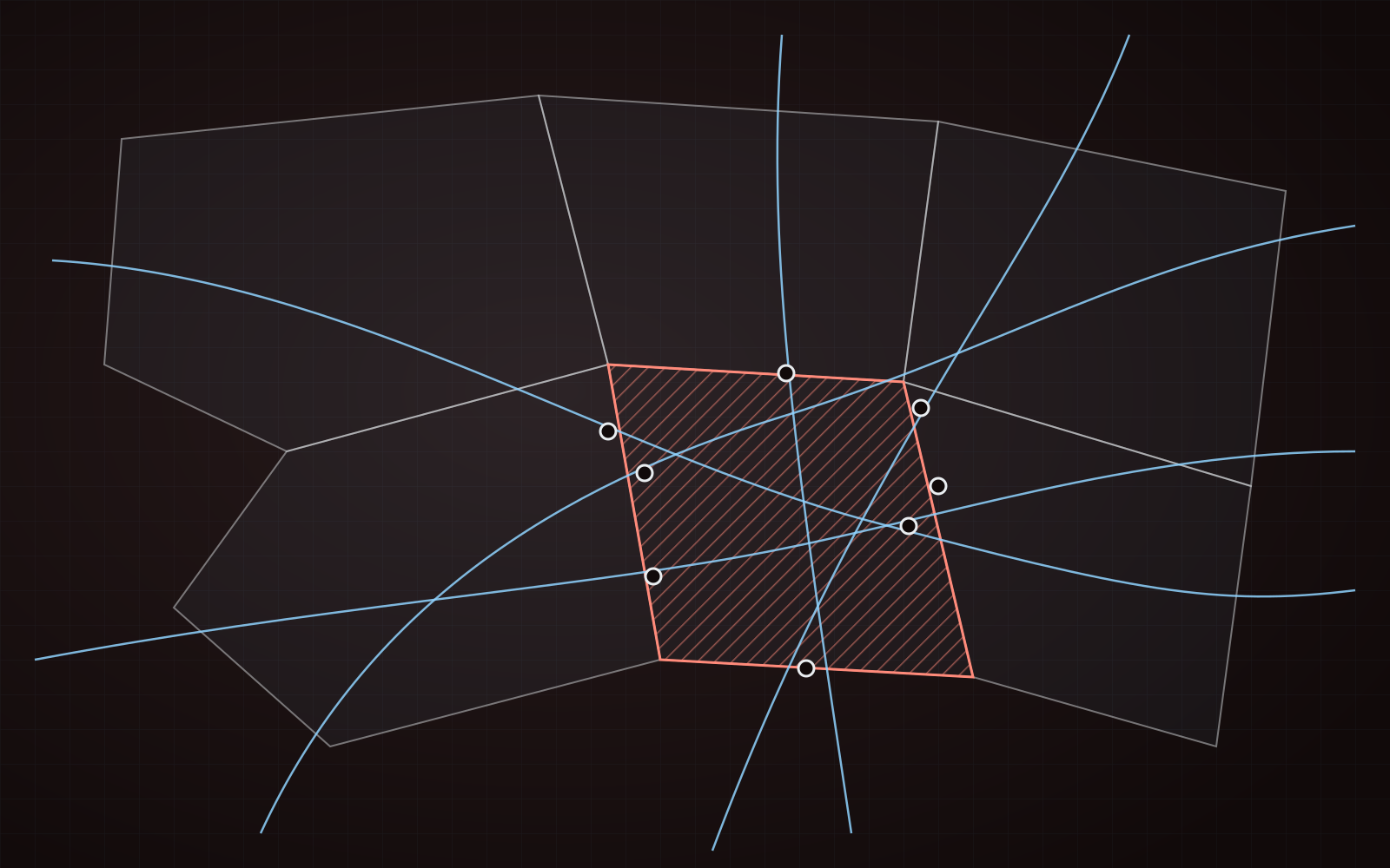
Each sector is the Voronoi cell of a generator point, so a candidate sectorisation is just the list of generator positions: a latitude and a longitude for each of the five points, ten variables in total, kept inside the extent of the FIR. The genetic algorithm moves these points.

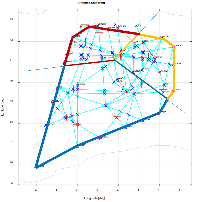
Single objective: balancing sector area

As a first objective we balanced the sector areas, minimising their relative standard deviation:

where $\sigma_A$ is the standard deviation of the five sector areas and $\bar{A}$ their mean. We ran it with a genetic algorithm written for the course and with MATLAB’s ga.

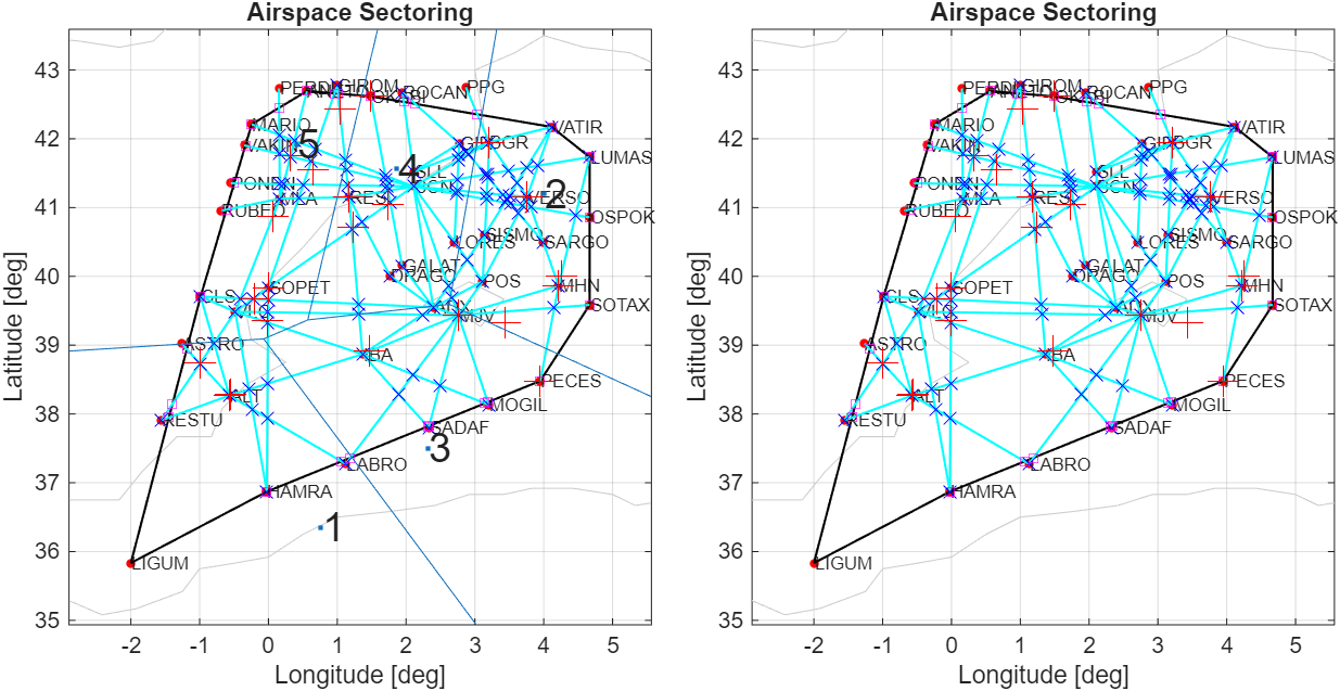
Both balanced the areas well, and both showed the problem with optimising one parameter alone: the number of aircraft per sector went from 0 in one sector to 25 in its neighbour.

Tuning the genetic algorithm

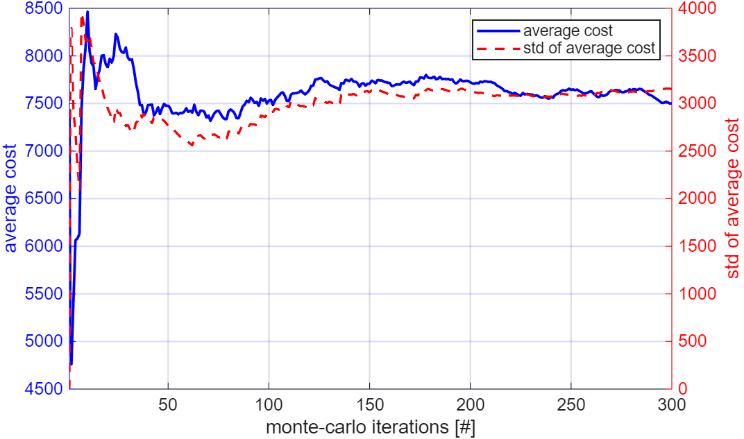
Population size and number of generations decide how well a genetic algorithm converges and how long it takes. We first found how many repeated runs give stable statistics, by plotting the mean and standard deviation of the best cost against the number of Monte Carlo runs, and settled on 150 runs per setting.

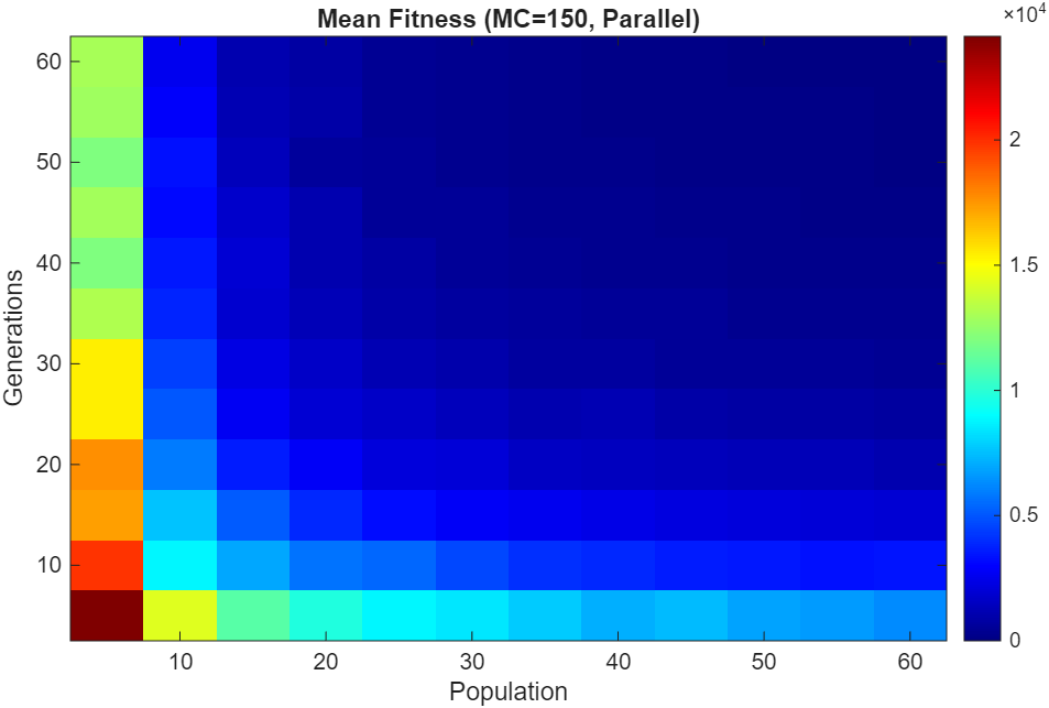
We then mapped the mean fitness over a grid of population sizes and generation counts. Fitness improved with both, with diminishing returns: beyond about 60 individuals and 60 generations the gain was marginal while the cost kept growing. Two settings near the bend were carried forward: 50 generations with a population of 30, and 50 generations with a population of 50.

Two objectives and the Pareto front

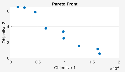
The third part balanced two conflicting objectives at once: the spread of sector areas and the spread of aircraft counts between sectors, both measured by their standard deviation. We built the Pareto front in two ways:

• a weighted sum of the two objectives with a parameter $\alpha$, solved as a single-objective problem for a range of $\alpha$ values, keeping the non-dominated solutions;
• a true multi-objective genetic algorithm, NSGA-II, through MATLAB’s gamultiobj.

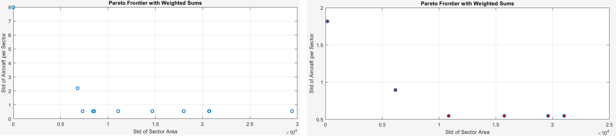
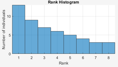
The setting with 50 generations and a population of 30 gave the more useful front: curved, so the region of best compromise is easy to see, with a rank histogram showing the population had converged. With a population of 50, the population stayed more mixed after the same number of generations and the front was less well defined.

The weighted sum gives a smoother, simpler curve but can miss parts of the front, depending on the range and spacing of $\alpha$. NSGA-II gives a denser set of solutions and a fuller picture of the trade-off.